Every content here is my original work.Creative Commons Licence
Universitas Scripta is licensed under a Creative Commons Attribution-NonCommercial-NoDerivs 3.0 Unported License.
Your cookies may be used by Google and mathjax. See Google's privacy policy.
Showing posts with label Physics. Show all posts

Wednesday, 3 August 2022

Solution to the high frequency damping problem by low-pass filter

Previously, I showed you how the simplest R2R DAC-generating step-functioned signals is damped by the low-pass filter from the original ideal signal, and this is fundamental not artificial, so no one can regenerate the original signal.

Solution to this is, of course, studied by many people. As I hinted in the previous article, I thought that to interpolate and to regenerate the original signal, I may have to do Fourier transform and then inverse Fourier transform. I started to search in such direction. And then, I found a great article teaching the sinc interpolation.

http://www.ipol.im/pub/art/2011/g_lmii/revisions/2011-09-27/g_lmii.html

sinc function is a great "Fourier-styled smooth" impact function. Only t=0 node is excited and other nodes are zero, so if this function is digitally sampled, that would look like just a impulse. Also, this function has all the frequencies fully from 0 to the Nyquist frequency. This function definitely will connect the dots smoothly, fully mobilizing all the lower-than-Nyquist frequencies.

If you think that this is too brick wall -- see the DAC datasheet and you can see the brick wall oversampling style, and this rings too much -- , then we can do more smooth. For example, suppressing the ringing by the normal distribution, \(e^{-t^2/\sigma^2} \mathrm{sinc} \pi f_s t\), makes the frequency response more smooth.

Friday, 27 May 2022

Hi-res is absolute necessity

People tend to forget the audio is analogue. Some says that only 44kHz is necessary because of Nyquist theorem. However this only proves that there is one-to-one correspondence between the original discrete data set and its Discrete Fourier Transform only if we eliminate the higher frequencies in the inverse Fourier transform. This does not mean that the discretely sampled data guarantees to be recovered as its original analogue wave function by the conventional audio circuit with low-pass filter.

Simple thought experiment reveals the contradiction in the 44kHz-sufficiency believers. 22kHz wave is annihilated in the sampling by 90-deg phase shifts. 11kHz is also only guaranteed to be sampled at least 1/sqrt(2) by amplitude.

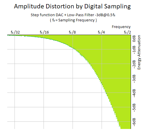
In this article, I simulated DAC generating step function signals followed by an analogue first-order low-pass filter with its cut-off at the Nyquist frequency. The plot shows the average energy of the regenerated output analogue signal compared to the original conceptual sine wave to be sampled.

As I argued before, and some of audiophiles believe, the 24/192 satisfies the 1dB distortion threshold. To satisfy 1% (0.08dB) distortion threshold, we need to go 24/768. Remember that the human hearing function is not that attenuated at the higher frequency.

We can display frequency response of the low-pass filter we applied layered over the plot as orange. However, be careful that you cannot divide the attenuation into the contribution from the filter and the theoretical contribution. If you do a little thought experiment, you can easily realise that the theory already says that the maximum attenuation at fs/4 is -3dB, which is close to the total attenuation in the plot. The additional attenuation comes from the shape smoothing from the step-shaped original wave shape.


Sunday, 1 May 2022

계산없이 배우는것은 없다!

이해란 무엇인가. 학습이다. 학습이란 무엇인가. 무수한 사례들과 correction에 의해 학습회로가 뇌속에 추상회로를 형성하는 과정을 말한다. 자전거를 책만 보고 잘 탈 수 있나? 수영은? 애초에 걸음마도 수없이 넘어져봐야 비로소 똑바로 할 수 있는 것이다. 매트릭스같이 데이터를 뇌 속으로 바로 쏴준다고 해도 학습은 불가능할지 모른다. 학습이란 '나'라는 배경, 주변환경, 자아를 가진 사람이 '나'에 맞게 주변 환경을 인식하면서 생기는 것이다. 다른 사람의 자전거 주행 데이터를 내 뇌속에 집어넣는다로 해서 잘 타지는 것이 아니라 오히려 더 잘 넘어지게 될 것이다.

그런데, 왜 과학은 누군가 제대로 설명만 해주면 이해한다고 생각하는 것인가? 초등학교 때 수없이 사칙연산을 연습하던 기억은 나지 않는 것인가? 당신은 정말 '더하기' '곱하기'를 '이해'하나? 선생님의 무수한 X표에 의한 교정으로 당신은 우리 사회가 합의한 연산과 같은 결과가 나오는 회로를 머릿속에 갖추게 되었을 뿐이다. 우리는 이를 '이해한다'로 가정하고 넘어가기로 하였다.

단순히 설명에 의해 이해하게 되는 것은 기존의 개념을 이용해서 설명할 수 있을 때 뿐이다. 즉, 당신이 누군가의 설명을 알아들었다면 그것은 새로운 것을 배운것이 아니다. 단지 새로운 조합을 알게 되었을 뿐. 완전히 새로운 것에 대한 학습을 하려면 당신은 두가지가 필요하다. 1. 무한한 연습과 그리고 2. 벌.

당신이 틀렸다고 누군가 이야기 해줄 수 있는 환경에서만 당신은 배울 수 있다. 단순히 책을 읽는다고 배울 수 있는 것이 아니다. 당신이 정말 과학에 문외한인데 책을 열심히 읽고 고민해서 뭔갈 이해한것 같다면 내 이야기를 들어보길 바란다. 우리 전문가들도 같은 과정을 초등학교, 중학교 때 거쳐왔으니까.

일단 책을 읽는다. 새로운 단어, 개념이 등장하기 때문에 당신은 자기가 알고 있는 것을 이용해서 어떻게든 끼워맞춘다. 그리고 당신 머리 속에서 모순이 없는것 같으면 납득하게 된다. 문제는 여기에 있다. 제대로 커리큘럼을 받는 학생들은 이 멍청한 개념을 가지고 숙제나 시험을 치게 된다. 그리고 형편없는 점수를 받고 나면 자신이 완전히 잘못 이해했다는 것을 알게 된다. 수학적으로 아주 명쾌하고 단순한 개념을, 인간이라는 오만한 존재의 '이해'라는 틀에 맞추기 위해 완전히 복잡하게 꼬아서 오해하고 있었음을.

이 과정을 16년간 겪고 나면 비로소 물리학의 '개념'이라는 것에 어느 정도 익숙해지게 된다. 계산과 개념이 동떨어진것처럼 얘기하는 사람이 있다. 계산만 많이 해봤지 제대로 이해하지 못하는거 아니냐고. 이건 잘못된 말인것 같다. 계산없이 이해할 수 없다. 둘은 같이 가는 것이다. 정확한 수학을 해보지 않고 과학을 설명한다는 것은 어불성설인 것이다.

경험이란 정말 중요한 것이다. 아무리 조선시대 사람에게 전기를 설명해도 이해할 수 없지만, 오늘날 사람들에게 전기란 너무 당연한 것이다. 하지만 그것조차 그저 익숙한 것일뿐 물리학적 관점에서는 이해하지 못하는 것과 별반 차이가 없을 것이다. 학과과정을 겪고나서야 전기이론을 세운 사람들에 사고과정에 다가갈 수 있을 뿐이다. 실제 보빙사에게 아무리 전기에 대해 설명해주어도 알아듣지 못했다는 이야기를 생각해보라. 마찬가지로, 과거 사람에게 자동차에 대해 설명해주어도 그 사람들은 아무리 똑똑한 사람이어도 알아듣지 못한다. 현대 사람들은 자동차에 대해 이해하지 못하여도 태어났을 때 부터 봐왔기에 자동차의 존재에 대해 직관적으로 이해할 수 있다. 과거 사람에게 자동차에 대해 논하면 그나마 가장 똑똑한 사람은 자동차안에 말이 있다고 생각할 것이다. 이게 뭐 비유적인 표현으로서 어느 정도 넘어갈 수 있다고 생각한다면야 모르겠지만, 이내 그 과거 사람은 이러한 오류를 저지를 것이다 '말에게 풀을 먹여야지'

그러니 제발 물리학을 아마추어로라도 배우고 싶으신 분은 그냥 대학에 진학하기를 추천한다. 하다못해 차선책으로 과외하시는 분도 많더라. 제발 혼자 이해하려고 하지 마라. 그리고 선생님이 설명을 잘 못해도 그러려니 해라. 자전거 타는 법을 잘 설명하는 사람이 있던가? 자전거 타는 법을 몸이 익히도록 하는 것이 중요한 것이다. 설명을 잘 하는게 중요한게 아니다. 마찬가지로 대부분의 교수들은 당신이 열심히 연습하다가 넘어졌을 때, 곤경에 처했을 때 도움을 줄 수 있는 존재이지, 설명으로 감탄케 하는 존재가 아니다. 그러나, 처음에 설명할 때 잘 듣고, 넘어졌을 때 도움을 청하라. 이해가 될 때까지 질문하라. 스키를 타기 전에 강사말을 잘 듣고, 일단 타기 시작하면 잘 넘어져야하는것과 같은 원리이다.

Monday, 29 November 2021

빨간책 신봉자들을 혐오하는 이유

예전부터 소위 '물리 동인계'에서는 파인만 강의록이 주요 텍스트북이 되어 있는 모양이다. 최근 유튜브가 뜨면서 그런 사람들이 유튜브에도 나타나고 있는 모양인데, 예전부터 그 빨간 책에 손이 잘 가지도 않았지만, 요새 그 책을 신봉하고 떠받드는 인간들을 보면, 그 책만 읽고 자기가 물리의 대가라고 착각하는지 뭔지 모르겠지만, 자기보다 잘 모르는 소리 하는것 같은 사람이나, 자기가 생각하는거랑 다른 얘기를 하는 사람에게 공격을 하는 사람이 많다. 그 책이 비교적 사람들에게 가장 많이 알려지고 진입장벽이 낮기 때문에 그런 것이 아닐까 싶다. 하지만 기본적인 배움의 자세와 예의도 되어 있지 않은 인간들이 주로 읽는 책이라고 하니 정이 가지 않는것도 사실이다. 만약 파인만 강의록이 아주 놀랍다고 생각하는 사람들은, 당신들이 그만큼 물리적인 개념에 익숙치 않았었다는 사실을 깨닫는 것이 좋다. 물리 공부를 조금이라도 해본사람들이 그 책을 본다면, '당연한것들을 좀 재밌게 써놨네' 정도로 생각할 것이다. 또한, 하나의 책에 감탄을 느꼈다는 것은, 그만큼 여러가지 다른 의견들이나, 같은 주장이라도 다른 식으로 쓰여진 문장에 전혀 익숙치 않다는것, 그리고 그 분야를 공부함에 있어서 필요한 수년간의 경험이 부족하다는 뜻일것이다. 당신이 수십년간 textbook을 보고, 문제를 풀어보고, 그리고 학교에서, 혹은 정답지에서 당신이 틀렸다는 사실을 배울때마다, 당신이 책의 '문장'을 보고 멋대로 오해하면서 습득한 추상적인 개념과 이미지가 수정되며 망치질 당하며, 그렇게 학계에서의 '대부분의' 공통된 개념이 당신의 머리속에도 비슷하게 자리잡게 되는것이다. 추상적인 개념을 타인에게 전달하는것은 매우 어렵다. 구체적인 사례에서의 '잘못됨' '충돌'을 통해 교정됨으로서만이 서로 비슷한 개념을 공유하는것을 가능케 하는것이다. 그렇기 때문에 제대로된 학교도 다니지 않고, '이 책을 보고 감명받았다'든가하는 인간들이 혼자서 파고들기 시작하면 결국 이상한 사이비학자가 되는것이다. 학계를 보고 폐쇄적이다 권위적이다 하지만, 그럴 필요가 있는것이다. 적어도 누구나 학계에 들어올수는 있다. 당신이 돈을 내고 학교를 제대로 다니고, 교수들의 말에 귀를 열고 받아들일 자세만 되어있다면 말이다.

잘난척하는 인간들보고 입닥쳐라고 하는것도 문제가 있다고 본다. 실수하는 인간들에 대한 관용이 없다면 새로 진입하는 사람들을 막는 일이 된다. 그리고 이 세상 누구도 100% 옳은 말을 하는 인간은 없으며, 옳음이 존재하는지조차 의문이다. 하지만 적어도 당신이 생각하는것과 다르다고 상대를 인신공격하는 것만은 그만두었으면 한다. 무엇보다도 제대로 아는 사람은 상대가 멋모른소리를 한다고 화내지 않는다. 왜냐하면 그 사람 주변에는 자기보다 모르는 사람들만 봐왔을 것이기 때문이다. 관심을 가져줘서 기뻐할지언정 화는 내지 않는다. 당신이 다른사람의 말을 보고 화가 난다면, 당신이 그것에 대해 잘 안다고 뽐내고 싶어하기 때문이거나, 당신이 그것에 대해 이론적으로는 잘 모르지만 경험적으로 스스로 만들어낸 어떠한 법칙에 대해 부정당했을때 자신에 대해 부정당한다고 착각하기 때문일 것이다. 하지만, 이미 그런 법칙에 반하는 사례를 당신 스스로도 수차례 경험했을 것이며, 그렇기 때문에 더 화가 날것이다. 미안하지만, 경험없는 이론도 쓸모가 없지만, 이론없는 경험도 쓸모가 없기는 마찬가지이다. 이것 또한 사이비 이론을 만드는 한 방법인것이다.

진정한 학자는 상대가 내가 잘 모르는 소리를 했을 때, 그 사람이 쓰는 언어의 의미를 파악하려고 노력한다. 학문에서는 용어의 정의가 우선이며, 이것은 분야마다 다르기 때문에 그것을 파악하는 것이 우선이다. 그러고나서는 그 용어를 이용하여 설명하고자 하는 추상적인 개념을 얻고자한다. 토씨하나하나 따지는것이 아니라.

어쨌든 지금까지 봐온 인간군상들을 보자면, 반혐오주의를 외치는 혐오주의자, 반지성주의를 혐오한다고 외치는 반지성주의자들이었다. 어찌나 거울처럼 똑같던지. 아니, 오히려 한국에서는 저런 안티-안티가 원래의 안티보다 더 숫자가 많아져서 오히려 더 안좋아보인다. 어그로가 쉽께 끌리는 민족이라 그런지. 대부분의 사람들이 자기 머리로 생각하지 않고 다수의 흐름대로 생각하는 사람들이라 그런것일 것이다. 그러면서 본인 머리로 생각하고 있다고 착각하고 있는 사람들. 이유를 물어보면 그저 화내는 사람들. 그런 사람들이 인구의 대부분일 것이다. 남들보고 닥치라고 하는 사람들. 반반지성주의를 가장한 반지성주의자들. 당신들이야말로 닥쳐줬으면 한다.

Wednesday, 2 December 2015

Is there the reference frame of the universe?

The Newtonian mechanics, the beginning of physics, is based on Galilean relativity: every inertial frame has the same laws of physics and there is no reference frame. But, is it?

Development of electromagnetism in 19th century discovered that the speed of light is universally constant in our universe. This implies that the Galilean relativity does not work anymore: 100 mph ball thrown on a truck running 100 mph is no longer 200 mph! Instead, there is special way of adding speeds to preserve the speed of light, which is the special relativity.

All these theories are developed in belief of relativity i.e. no reference frame, and Einstein's relativity shows time dilation, length contraction, and blue/red-shift: if we are getting closer to the light source, it seems more bluer than its original light, and if we are getting farther, it seems more red-er. We call it relativistic Doppler effect. This is the natural consequence of the relativity.

If it is the natural consequence of the relativity, and if there is no reference frame, then the universe must be isotropic just as we see on the earth even if we are speeding relativistically away from our home. Is it?

We are having detected cosmic background radiation, the remnant heat from the big bang, which is uniform in any corner of the sky. If we are moving at speed of 99.5% of the speed of light away from our home, our clock is 10 times slower than our home, and we can detect 10 times stronger the radiation in the moving direction, and 10 times weaker in the opposite direction. So, if we have enough fuel to accelerate to that speed, we can definitely take advantage of the 10-time time dilation, but we may not survive from the star radiation coming toward our windshield.

This phenomenon gives the exact reference frame: if we move away from that frame, the universe may not look isotropic anymore. This makes us ask a question: where did the relativity come from?

Theoretically, of course, we can make a theory, a set of laws of physics, which guarantees the relativity, but the solution of the equation being not. But the relativistic principle itself came from the empirical conclusion. Galileo might experiment many times about motion, momentum, inertia, and relativity. It is believed so strongly because it has never been disproved, but we cannot prove that it is right assumption. A postulate can never be proved.

So far, every modern experiments prove the Einstein's relativity to be right. However, we are already facing a contradiction: black hole problem in General relativity. Science is waiting for another big wave following Newton, and Einstein.

Saturday, 22 November 2014

Entrance to the black hole: Talk with Frolov

I am quite unsatisfied with Hollywood movie 'Interstellar' on its physical description as well as its plot. Even not in physics, one blogger described well about what should be considered in the movie.
http://vegaseul.blog.me/220180270224

I want to talk about basic issue which is more certainly confidently to be said true than Thorne's 'picture'. In this article, I want to talk about 'when an object is to be said "absorbed" to the black hole'. I have discussed about this problem with Valeri Frolov in the last winter school, and he introduced the solution which is widely accepted among the black hole physicists. Well, simply said, 'under the Planck length, we cannot distinguish from the horizon'.

Let's think about it more in quantum sense. As an object approaches to the horizon, the radiation or any emission including reflection which may come from the object red-shifts. Thus, for the Schwarzschild at the Schwarzschild frame, the object at \(r=2M+l\) may be seen with redshift of factor \(\sqrt{\frac{l}{2M}}\). If the seen frequency is less than the inverse of the lifetime of the universe which cannot be lived longer by any observer, the energy is totally quantum and out of conservation of energy which now can be explained as a part of the black hole. In the different, the object's frame, the observation is very short time near horizon. A short moment passing the horizon may corresponds to eternity in the Schwarzschild frame. Any observation from the asymptotic rest frame should be committed by emission in such short (proper) time which prevents exact energy measurement. This gives different condition from the 'Planck length' explanation which mentioned in earlier passage, but this makes more sense as we cannot define 'length' well if we still believe equivalence principle.

This also gives somewhat similar intuition with CFT scattering amplitude and particle counting problem. In theory with no mass gap, particle counting is hardly defined. In this situation, as system goes near horizon, energy goes to zero which effectively make the energy gap converge to zero.

Monday, 3 November 2014

How to use easiest version control system

When you lost your data or history by crash or accidently saving process, you might be very frustrated. People usually use Dropbox, but Dropbox cannot sync into custom directories, multiple history branches, and massive collaborators. I will introduce intuitive guide to one of version control system 'git', which supports multi-branch, multi-collaborator projects.

The only point people might hesitate may be that git is open-source-based: mostly you are forced to share your sources you uploaded on the git repositories. There is good service which avoid this license: bitbucket, which gives up to 5 free private repositories per user. This service is provided by Atlassian who also provides git client program with intuitive user interface: SourceTree.

First, you should make your repository on the server e.g. bitbucket. Then, you should clone your server repository into a blank directory of your local disk. When you change your local file, the sourcetree app shows what is changed, and you can 'commit' to make a node to the history line. 'push' pushes the nodes to the server and make changes to the server which are shared to all collaborators. If there are conflicts between collaborators, it automatically merges, or you can fix it in your way. When you transfer into another branch, data of the local repository changes, so you should be aware of it.

Monday, 22 September 2014

Rarita-Schwinger Fields

Rarita-Schwinger term which may be satisfied by spin-3/2 fields may be \[\mathcal{L}=\bar{\psi}_\mu \left(\frac{i}{2}\gamma^{\mu\nu\lambda}\partial_\nu - \frac{m}{4}\gamma^{\mu\lambda}\right)\psi_\lambda\] Signs and coefficients may depend on notations.
Be aware that the product of vector index and spinor index may split into two representations: spin-3/2 and spin-1/2. \[V\otimes S = R\oplus S\] Specifically expressed in highest-weight representations, \(1\otimes\frac{1}{2}=\frac{3}{2}\oplus \frac{1}{2}\), especially in 4-dimensions, \(\left(\frac{1}{2},\frac{1}{2}\right)\otimes\left(\frac{1}{2},0\right) = \left(1,\frac{1}{2}\right)\oplus \left(0,\frac{1}{2}\right)\). Spinor degrees of freedom may be found if we consider trace component \(\gamma^\mu \psi_\mu\); from the Rarita-Schwinger term, if you combine \(\gamma^\mu \psi_\mu\) as a spinor, the spinor may satisfies Dirac equation, so the trace may have spin-1/2 representation. To express spin-3/2 representation, we may introduce trace-less condition to the vector-spinor-indiced field.\[\gamma^\mu \psi_\mu=0\]
In \(d\)-dimensions, vector representation has \((d-2)\) degrees on-shell and \((d-1)\) off-shell. Dirac spinor has complex \(2^{[d/2]}\) degrees off-shell and real \(2^{[d/2]}\) degrees on-shell. The constraint (traceless condition) annihilates degrees as many as the spinor degrees. Off-shell degrees are \((d-1)n\) where \(n\) is the spinor degrees \(2^{[d/2]+1}\) in real degree. On-shell degrees are \((d-2)n-n=(d-3)n=(d-3)2^{[d/2]}\).
  • http://www.ift.unesp.br/users/nastase/sugra.pdf
  • Weinberg

Wednesday, 25 December 2013

Penta-denominator Integrals

\[\int\frac{d^dk}{(2\pi)^d}\frac{d^dl}{(2\pi)^d} \frac{1}{k^2 (k-p)^2 l^2 (l-p)^2 (k-l)^2}={{_{0,0}F_0}}(d)\, (p^2)^{d-5}\]\[\int\frac{d^dk}{(2\pi)^d}\frac{d^dl}{(2\pi)^d} \frac{k_\mu}{k^2 (k-p)^2 l^2 (l-p)^2 (k-l)^2}={{_{1,0}F_0}}(d)\,p_\mu (p^2)^{d-5}\]\[\int\frac{d^dk}{(2\pi)^d}\frac{d^dl}{(2\pi)^d} \frac{k_\mu k_\nu}{k^2 (k-p)^2 l^2 (l-p)^2 (k-l)^2}={{_{2,0}F_0}}(d)\,p_\mu p_\nu (p^2)^{d-5}+{{_{2,0}F_1}}(d)\,\hat{\delta}_{\mu\nu}(p^2)^{d-4}\]

Thursday, 2 May 2013

Possibility of Charge Addition to the Reissner-Nordstrom Black Hole


     The Reissner-Nordstrom black hole has background field of metric
\[g_{\mu\nu} = \mathrm{diag}\left\{-\left(1-\frac{r_s}{r} + \frac{r_Q^2}{r^2}\right),\,\left(1-\frac{r_s}{r} + \frac{r_Q^2}{r^2}\right)^{-1},\,r^2,\,r^2\sin^2\theta\right\}\]
where
\[r_s = 2GM;\;\; r_Q^2 = \frac{GQ^2}{4\pi}\]
and of electromagnetic field
\[A_t = \frac{Q}{4\pi r}\]
Then, the geodesic is determined by the action
\[S=\int d\tau\left[-m\sqrt{(1-\frac{r_s}{r} + \frac{r_Q^2}{r^2})\dot{t}^2 - \frac{1}{1-\frac{r_s}{r} + \frac{r_Q^2}{r^2}}\dot{r}^2 - r^2\dot{\phi}^2}+\frac{qQ}{4\pi r} \dot{t}\right]\]
assuming the motion is on the plane \(\theta=\frac{\pi}{2}\),
where the normalisation of the proper time is determined by
\[\sqrt{\cdots} \equiv \sqrt{(1-\frac{r_s}{r} + \frac{r_Q^2}{r^2})\dot{t}^2 - \frac{1}{1-\frac{r_s}{r} + \frac{r_Q^2}{r^2}}\dot{r}^2 - r^2\dot{\phi}^2}=1\]

     We may, first, obtain the equation of motion in angle.
\[\frac{\delta S}{\delta \phi} = -\frac{d}{d\tau} \frac{mr^2\dot{\phi}}{\sqrt{\cdots}} = -\frac{d}{d\tau} mr^2\dot{\phi}=0\]
So, we have found a constant of motion, angular momentum, which should be defined as
\[L\equiv m r^2\dot{\phi}\]
Now, we may take variation in direction of time.
\[\frac{\delta S}{\delta t} = -\frac{d}{d\tau} \left[\frac{-m () \dot{t}}{\sqrt{\cdots}}+\frac{qQ}{4\pi r}\right] = -\frac{d}{d\tau} \left[-m () \dot{t}+\frac{qQ}{4\pi r}\right] = 0\]
with the shorten expression
\[() \equiv \left(1-\frac{r_s}{r} + \frac{r_Q^2}{r^2}\right)\]
This equation of motion is also cyclic so we may define the constant of motion
\[E = -m () \dot{t}+\frac{qQ}{4\pi r}\]

     The only remaining equation of equation is related to \(r\), but we may alternate the equation to the normalisation condition, conserving the degree of freedom.
\[1= \cdots = () \dot{t}^2 - ()^{-1} \dot{r}^2 - r^2 \dot{\phi}^2 = \frac{1}{m^2 ()}\left(\frac{qQ}{4\pi r} -E\right)^2-()^{-1} \dot{r}^2-\frac{L^2}{m^2r^2} \]
We may manipulate the equation as similar to the classical mechanics.
\[\frac{1}{2}m \dot{r}^2  + \frac{L^2}{2mr^2}\left(1-\frac{r_s}{r}+\frac{r_Q^2}{r^2}\right) - \frac{1}{2m}\frac{q^2Q^2}{16\pi^2r^2} + \frac{1}{m} \frac{qQE}{4\pi r} = \frac{E^2}{2m}-\frac{m}{2}()\]
By special relativity, you may find \(\frac{1}{2}m \dot{x}^2 = \frac{E^2}{2m}-\frac{m}{2}\) where \(E\) is the total energy of a particle, so \(E\) is the asymtotic energy of the test particle, in this problem.
Thus, this equation is in analogy to the energy conservation law in classical mechanics.

     To simplify the situation and ease to enter the black hole, we may consider the situation \(L=0\).
Then, this seems to be a system with potential \(V(r) = -\frac{q^2Q^2}{32\pi^2 m r^2}+\frac{qQE}{4\pi mr}\), but this term itself contains the total energy \(E\) so we have to consider more carefully. First, from the shape of the potential, we may guess that the test particle may fall to the centre if the particle just overcome the threshold. i.e. \(V(r) = \frac{E^2}{2m}-\frac{m}{2}\) should have no solution. However, the solution is \[ r = \frac{qQ}{4\pi (E\mp m)}\]which always exists, considering the absolute condition \(E\geq m\). Thus, the particle always bounce back to the infinity at the outer critical point \[r = \frac{qQ}{4\pi (E-m)}\]
Not to enter inside of the horizon, the criterion is thus
\[\frac{E-m}{q} \leq \frac{\sqrt{M^2 + \frac{Q^2}{4\pi G}}-M}{Q}\]


For further study: I'll note here http://arxiv.org/abs/1304.6474 which is a part of my project here. I may list tasks to determine charged black hole stability and radiation
*particle generation in strong electric field
*decay rate of particle-anti-particle pair in terms of gas density

Friday, 18 January 2013

4-D Clifford Algebra with (-1,1,1,1) signature

Weyl Basis: \[\gamma^0=\begin{bmatrix}0&-1\\1&0\end{bmatrix};\; \gamma^i=\begin{bmatrix}0&\sigma^i\\\sigma^i&0\end{bmatrix}\]
Dirac Basis: \[\gamma^0=\begin{bmatrix}i&0\\0&-i\end{bmatrix};\; \gamma^i=\begin{bmatrix}0&\sigma^i\\\sigma^i&0\end{bmatrix}\]
Majorana Basis: \[\gamma^0=\begin{bmatrix}0&i\sigma^2\\i\sigma^2&0\end{bmatrix};\; \gamma^1=\begin{bmatrix}-\sigma^3&0\\0&-\sigma^3\end{bmatrix};\; \gamma^2=\begin{bmatrix}0&-i\sigma^2\\i\sigma^2&0\end{bmatrix};\; \gamma^3=\begin{bmatrix}\sigma^1&0\\0&\sigma^1\end{bmatrix};\;\]
\[\gamma^\mu_{\text{Dirac}}=\begin{bmatrix}\frac{1}{\sqrt{2}}&\frac{i}{\sqrt{2}}\\\frac{i}{\sqrt{2}}&\frac{1}{\sqrt{2}}\end{bmatrix}\gamma^\mu_{\text{Weyl}}\begin{bmatrix}\frac{1}{\sqrt{2}}&\frac{i}{\sqrt{2}}\\\frac{i}{\sqrt{2}}&\frac{1}{\sqrt{2}}\end{bmatrix}^{-1}\]

Saturday, 14 July 2012

Dirac Fields (1)

Dirac Basis

The wave equation for integer spins are already known as Klein-Gordon equation: \[\partial^2\phi +m^2\phi = 0\]We may develop half-ranked field to be \[(i\gamma^\mu\partial_\mu-m)\psi = 0\tag{1}\]when \[(\partial^2 +m^2)\psi = -(i\gamma^\mu\partial_\mu+m)(i\gamma^\mu\partial_\mu-m)\psi\]To satisfy the last equation, the Clifford algebra condition must be satisfied.\[\{\gamma^\mu,\gamma^\nu\} = 2\eta^{\mu\nu}\]Also the Lagrangian which derives the Dirac equation \((1)\) can be written as \[\mathfrak{L} = \bar{\psi}(i\not{\partial}-m)\psi\]where \(\not{\partial}=\gamma^\mu \partial_\mu\). Then, we can see that the U(1) charge is \[\int \bar{\psi}\gamma^0\psi \,d^3x\]and usually we demand it to be \(\int \psi^\dagger\psi\, d^3x\) to guarantee finiteness so \[\bar{\psi} := \psi^\dagger\gamma^0\]

     Any basis of gamma matrices and their following theories are all equivalent, so first the Dirac basis is taken which is handy in nonrelativistic case.\[\gamma^0 = \begin{bmatrix}1&\\&-1\end{bmatrix};\quad\gamma^k = \begin{bmatrix}&\sigma^k\\-\sigma^k&\end{bmatrix} \]There is also Weyl basis which is written \[\gamma^0 = \begin{bmatrix}&1\\1&\end{bmatrix};\quad\gamma^k = \begin{bmatrix}&\sigma^k\\-\sigma^k&\end{bmatrix} \]

Eigenspinors

As gamma matrices are constants, the plane wave solution \(k_\mu = i\partial_\mu \Rightarrow \psi \sim e^{-i k_\mu x^\mu}\) can also be a solution for the Dirac equation. By applying the solution to the equation, the equation may transform into momentum space. Then, by producting \(\gamma^0\) to the whole equation,
\[k^0\psi =\gamma^0( \vec{\gamma}\cdot \vec{k} + m)\psi\]where \(k^\mu = (k^0,\vec{k})\). Here, the matrix on the right hand side is
\[\gamma^0( \vec{\gamma}\cdot \vec{k} + m) = \begin{bmatrix}m&\vec{\sigma}\cdot \vec{k}\\\vec{\sigma}\cdot\vec{k}&-m\end{bmatrix}\]The eigenvalue of \(k^0\) can be obtained as \(\pm\omega = \pm\sqrt{\vec{k}^2+m^2}\).

     For \(k^0=\omega\), \(\psi \sim \begin{bmatrix}m+\omega\\\vec{\sigma}\cdot\vec{k}\end{bmatrix}\). For \(k^0=-\omega\), \(\psi \sim \begin{bmatrix}-\vec{\sigma}\cdot\vec{k}\\m+\omega\end{bmatrix}\). Attached plane wave part, \[\begin{split}\psi &\sim \begin{bmatrix}m+\omega\\\vec{\sigma}\cdot\vec{k}\end{bmatrix}e^{-i\omega t + i \vec{k}\cdot\vec{x}} , \begin{bmatrix}-\vec{\sigma}\cdot\vec{k}\\m+\omega\end{bmatrix} e^{i\omega t + i\vec{k}\cdot\vec{x}}
\\&=\begin{bmatrix}m+\omega\\\vec{\sigma}\cdot\vec{k}\end{bmatrix}e^{-i\omega t + i \vec{k}\cdot\vec{x}}, \begin{bmatrix}\vec{\sigma}\cdot\vec{k}\\m+\omega\end{bmatrix} e^{i\omega t - i\vec{k}\cdot\vec{x}}
\\&=\begin{bmatrix}m+\omega\\\vec{\sigma}\cdot\vec{k}\end{bmatrix}e^{-ik_\mu x^\mu}, \begin{bmatrix}\vec{\sigma}\cdot\vec{k}\\m+\omega\end{bmatrix} e^{ik_\mu x^\mu}\end{split}\]These are the eigenfunction of the Dirac equation. As the first two and the second two have positive frequency and negative frequency respectively, the first eigenfunctions are usually interpreted as particle while the second are interpreted as antiparticle.

     Now, to normalise the functions in the same sense in the quantum mechanics, Noether charge may be normalised to 1. U(1) Noether charge of Dirac field is \[\int -\bar{\psi} i \gamma^0\delta\psi \,d^3x= \int \bar{\psi}\gamma^0\psi \,d^3x = \int \psi^\dagger \psi \,d^3x\]For both case, \[\psi^\dagger \psi = (m+\omega)^2 + (\vec{\sigma}\cdot\vec{k})^2 = m^2 + 2m\omega + \omega^2 + \vec{k}^2 = 2\omega(m+\omega)\]as \(m^2+\vec{k}^2 = \omega^2\).

     Finally, the Dirac eigenfunctions are \[\sqrt{\frac{m+\omega}{2\omega V}}\begin{bmatrix}\alpha_i\\\frac{\vec{\sigma}\cdot\vec{k}}{m+\omega}\alpha_i\end{bmatrix}e^{-ik_\mu x^\mu}, \sqrt{\frac{m+\omega}{2\omega V}}\begin{bmatrix}\frac{\vec{\sigma}\cdot\vec{k}}{m+\omega}\beta_j\\\beta_j\end{bmatrix} e^{ik_\mu x^\mu}\]where \(\alpha_i\)'s and \(\beta_j\)'s are the 2-component spinors for upper or lower space to handle \(2\times 2\) Pauli matrices and show the additional degrees of freedom which will correspond to classical spin.

     Or, the eigenspinors can be expressed with the scalar waves and spinors.\[u^{(i)}(\vec{k})\frac{e^{-ik_\mu x^\mu}}{\sqrt{2\omega V}}, v^{(j)}(\vec{k})\frac{e^{ik_\mu x^\mu}}{\sqrt{2\omega V}}\]so defined is\[u^{(i)}(\vec{k})=\sqrt{m+\omega}\begin{bmatrix}\alpha_i\\\frac{\vec{\sigma}\cdot\vec{k}}{m+\omega}\alpha_i\end{bmatrix};\quad v^{(j)} = \sqrt{m+\omega}\begin{bmatrix}\frac{\vec{\sigma}\cdot\vec{k}}{m+\omega}\beta_j\\\beta_j\end{bmatrix}\]and\[u^{(i+2)}(\vec{k})=v^{(i)}(-\vec{k});\quad v^{(j+2)}(\vec{k}) = u^{(j)}(-\vec{k})\]

Spin

Spinor indices come from space-time symmetry, so the space-time rotation may have corresponding transformation in spinor space. By considering the rotational transform \(x^\mu\rightarrow x^\mu+{\omega^\mu}_\nu x^\nu\) on the gamma matrices, which is a converter between spinor indices and space-time indices, we may find the spinor representation of rotation.

     First, we may consider general fields \(f(x^\mu)\), and then for the infinitesimal angle \(\omega\), the scalar field may transforms to \(f(x^\mu)\rightarrow f(x^\mu+{\omega^\mu}_\nu)\). Its generator may be \[L^{\mu\nu}=-i(x^\mu\partial^\nu-x^\nu\partial^\mu)\]so that \(f(x)\rightarrow e^{-\frac{i}{2}L^{\mu\nu}\omega_{\mu\nu}}f(x)\), and additional space-time indices may give other infinitesimal transforms.

     As the gamma matrices has 1 vector index and is (1,1)-rank tensor (linear operator) in spinor space, the matrices may transform, under rotation, \[\gamma^\mu \rightarrow U(\gamma^\mu+{\omega^\mu}_\nu\gamma^\nu) U^{-1} \]Be ware of that \(U\) is not guaranteed to be unitary. We may express with generators: \(U=e^{-\frac{i}{2}S^{\rho\sigma}\omega_{\rho\sigma}}\) (one half factor by analogy to \(L^{\mu\nu}\)). We expect that the gamma matrices is numeric tensor so invariant under such total transform. \[e^{-\frac{i}{2}S^{\rho\sigma}\omega_{\rho\sigma}}(\gamma^\mu+{\omega^\mu}_\nu\gamma^\nu)e^{\frac{i}{2}S^{\rho\sigma}\omega_{\rho\sigma}}=\gamma^\mu\]

     Applying Baker-Campbell formula \[e^X Y e^{-X}=Y +[X,Y]+O(X^2)\]gives the equation of commutators. \[\begin{split} &{\omega^\mu}_\nu\gamma^\nu-\left[\frac{i}{2} S^{\rho\sigma} \omega_{\rho\sigma}, \gamma^\mu+{\omega^\mu}_\nu\gamma^\nu \right] +O(\omega^2) \\&= {\omega^\mu}_\nu\gamma^\nu-\frac{i}{2} \left[S^{\rho\sigma}, \gamma^\mu \right]\omega_{\rho\sigma} +O(\omega^2) =0\end{split} \]As \(S^{\rho\sigma}\) has 2 space-time indices and has commutation relation with gamma matrices, the ansatz can be taken \(S^{\rho\sigma}=A \gamma^\rho \gamma^\sigma\). Then, as \[\left[\gamma^\rho\gamma^\sigma,\gamma^\mu\right]=\gamma^\rho\left\{\gamma^\sigma,\gamma^\mu\right\}-\left\{\gamma^\mu,\gamma^\rho\right\}\gamma^\sigma=2\eta^{\mu\sigma}\gamma^\rho-2\eta^{\mu\rho}\gamma^\sigma\]the equation becomes \[{\omega^\mu}_\nu\gamma^\nu-iA\left({\omega_\rho}^\mu\gamma^\rho-{\omega^\mu}_\sigma\gamma^\sigma\right) = {\omega^\mu}_\nu\gamma^\nu+2iA{\omega^\mu}_\sigma\gamma^\sigma=0\]As \(A=\frac{i}{2}\) satifies the equation, the solution may be \(S^{\rho\sigma}=\frac{i}{2}\gamma^\rho\gamma^\sigma\); however we demand the rotation generators to be antisymmetric generally, the solution may be antisymmetrised. \[S^{\rho\sigma}=\frac{i}{4}\left[\gamma^\rho,\gamma^\sigma\right]\]

     Therefore, Dirac fields transform by generator \(L+S\). Now we may see the eigenvalues of the total generator in the nonrelativistic limit to match the quantum mechanics. Before that, we may explicitly obtain the generator to calculate; here, in Dirac basis. \[\left[\gamma^i,\gamma^j\right]=-\left[\sigma^i,\sigma^j\right]=-2i\epsilon^{ijk}\sigma^k=-4i\epsilon^{ijk}S^{(Euclidean)}_k\]so\[S^{ij}=\epsilon^{ijk}S^{(Euclidean)}_k\]This is exactly the same with the familiar 3-d quantum mechanics. Thus, each upper and lower 2 component spinor in Dirac basis indicates the Pauli spinor for particle and antiparticle.

In Weyl basis, \[\left[\gamma^\mu,\gamma^\nu\right]=\begin{bmatrix}\sigma^{[\mu}\bar{\sigma}^{\nu]}&\\&\bar{\sigma}^{[\mu}\sigma^{\nu]}\end{bmatrix}\]
\[\left[\gamma^0,\gamma^i\right]=\begin{bmatrix}-2\sigma^i&\\&2\sigma^i\end{bmatrix}\]
\[ \left[\gamma^i,\gamma^j\right]=-\left[\sigma^i,\sigma^j \right]\]

Thursday, 28 June 2012

Wess-Bagger Weyl spinor notation

\[\eta_{\mu\nu}=\mathrm{diag}(-1,1,1,1)\]\[1=\varepsilon^{12}=-\varepsilon_{12}\]\[\varepsilon^{0123}=-\varepsilon_{0123}=1\]\[\psi^\alpha=\varepsilon^{\alpha\beta}\psi_\beta;\quad \psi_\alpha=\varepsilon_{\alpha\beta}\psi^\beta\]\[\psi^\dot{\alpha}=\varepsilon^{\dot{\alpha}\dot{\beta}}\psi_\dot{\beta};\quad \psi_\dot{\alpha}=\varepsilon_{\dot{\alpha}\dot{\beta}}\psi^\dot{\beta}\]\[\psi\chi=\psi^\alpha\chi_\alpha=-\psi_\alpha\chi^\alpha=\chi^\alpha\psi_\alpha=\chi\psi\]\[\bar{\psi}\bar{\chi}=\bar{\psi}_\dot{\alpha}\bar{\chi}^\dot{\alpha}=-\bar{\psi}^\dot{\alpha}\bar{\chi}_\dot{\alpha}=\bar{\chi}_\dot{\alpha}\bar{\psi}^\dot{\alpha}=\bar{\chi}\bar{\psi}\]\[(\chi\psi)^\dagger=(\chi^\alpha\psi_\alpha)^\dagger=\bar{\psi}_\dot{\alpha}\bar{\chi}^\dot{\alpha}=\bar{\psi}\bar{\chi}=\bar{\chi}\bar{\psi}\]\[\Psi_D=\begin{bmatrix}\chi_\alpha\\\psi^\dot{\alpha}\end{bmatrix}\]\[\gamma^\mu =\begin{bmatrix}&\sigma^\mu\\\bar{\sigma}^\mu&\end{bmatrix}\]\[\gamma^\mu =\begin{bmatrix}&\sigma^\mu\\\bar{\sigma}^\mu&\end{bmatrix}\]\[\sigma^\mu = (-1,\vec{\sigma});\quad \bar{\sigma}^\mu = (-1,-\vec{\sigma})\]\[\bar{\sigma}^{\mu\dot{\alpha}\alpha}=\varepsilon^{\dot{\alpha}\dot{\beta}}\varepsilon^{\alpha\beta}\sigma^\mu_{\beta\dot{\beta}}\]\[\mathrm{tr}\,\sigma^\mu\bar{\sigma}^\nu = \sigma^\mu_{\alpha\dot{\alpha}} \bar{\sigma}^{\nu\dot{\alpha}\alpha} = -2\eta^{\mu\nu}\]

Wednesday, 23 May 2012

Appendices: Natural unit constants

NameValueError
1 metre5. 067 730 94×106eV-12.2×10⁻⁸
1 kilogram5. 609 588 845×1035eV2.2×10-8
1 second1. 519 267 51×1015eV-12.2×10⁻⁸
1 Newton1. 231 618 15×1012eV28.8×10-8
Gravitational constant 4πG8. 429 98×10-56eV-21.2×10⁻⁴
Atomic mass 1u9. 314 940 61×108eV2.2×10-8
1 Kelvin = Boltzmann constant8. 617 332 4×10⁻⁵eV9.1×10-7
1 Ampere1. 244 064 71×103eV4.4×10-8
1 Coulomb1. 890 067 09×10186.6×10-8
Elementary charge e=√4πα0. 302 822 1208.8×10-8

Tuesday, 27 December 2011

On Construction of Energy-Momentum Tensors

We may think of continuum version of energy and momentum as we learned particle geodesic. We may define the flow of energy and momentum which is called energy-momentum tensor, and talks about its conservation. Also, just like defining the energy and momentum of electromagnetic field in classical electrodynamics, we may define the energy-momentum tensor of force fields, in way of conserving the whole energy-momentum tensor. Then, we may obtain the tensor for some specific cases: one particle, perfect fluid, spin-1 field, and thermodynamical gas of classical particles and photons; and confirm the consistency between statistical mechanics and relativistic fluid theory, and between gravitational theory and electromagnetic field theory.


Introduction

In classical mechanics, we found some conservative quantities which is called momentum. You may have defined the momentum with some conservative quantities by evolution of time in Newtonian mechanics, or you may have directly derived from the Lagrangian itself in canonical way.

     We will talk about the conservative quantities which corresponds to energy and momentum in continuum and its conservation law. Then, interaction may break the conservation and revise the conservation to the equation of motion. We may define the energy-momentum tensor of the interaction so that still the energy-momenum is conserved, as we defined Maxwell stress tensor in classical electrodynamics.


Conservative Quantities

You may understand well the conservative law of charged particles (fluid): \[\frac{\partial \rho}{\partial t} + \nabla\cdot(\rho\vec{v})=0\tag{1}.\] Here, we call \(\int \rho d^3 x\) the (conservative) charge and \(\rho \vec{v}\) the current. Under the Lorentz boost, we can find that the density \(\rho\) is not a proper scalar in the 4-D, but is magnified \(\gamma = (1-\beta)^{-1/2}\) times by the length contraction. So, using the proper density \(\rho_0 = \rho/\gamma\), the density in the local frame of fluid, the equation \(\mathrm{(1)}\) may be expressed as \[ \frac{\partial \gamma\rho_0}{\partial t} + \nabla\cdot(\gamma\rho_0\vec{v})=0 ,\] which also can be expressed with the 4-velocity \(u^\alpha\)  \[ \nabla_\alpha (\rho_0 u^\alpha ) = 0.\tag{2}\]Thus, we can understand that \(j^\alpha = \rho_0 u^\alpha\) should be called the proper 4-current in the same manner above, and the conservative charge is \(q = \int \rho d^3 x = \int j^0 d^3x\) for a flat time slice, in the special relativity. If we expand this naturally to the general relativity, the charge within an arbitrary time slice segment \(R\) may be defined as \(\int_R \rho(R)d^3x=\int_R j^\alpha dS_\alpha\).

     This proposal works well for non-mass charges such as electric charge as above, but mass-related quantities defined using above make some catastrophe. Analogy to above, we might define mass current \(\rho_0^\mathrm{(mass)}u^\alpha\), but this quantity is not an actual physical quantity. In a physical frame, only energy and momentum is an observable. Thus, we may define a current of energy and momentum density, the zeroth component of which may be the density itself.

     First, the zeroth component, the energy current may be considered. Consequent discussion may progress in the flat spacetime. The energy conservation may be written as: \[\frac{\partial \rho}{\partial t} + \partial_k (\rho v^k) = 0\tag{3}\]where \(\rho\) is the energy density. Distinctly from the electric example, the energy density may be transformed into \(\gamma^2\) magnified, one \(\gamma\) of which is from the length constraction and another one of which is from the 4-momentum transformation (mass increase), under the Lorentz transformation (\(\rho = \rho_0 \gamma^2\)). Thus, using the rest mass density \(\rho_0\), the equation may be expressed to \[\partial_\alpha (\rho_0 \gamma u^\alpha) = 0.\]As \(\gamma = u^0\) and generally the partial derivative is extended to the covariant derivative in the general relativity, the covariant form may be naturally \[\nabla_\alpha (\rho_0 u^0 u^\alpha) = 0.\]Then the zeroth component \(\rho_0 u^0 u^0\) is the energy density as we proposed.

     Second, we may remind the Navier-Stokes equation to write the equation of momentum conservation i.e. equation of motion in fluid[1,2]: \[\rho \frac{\partial v^k}{\partial t} + \rho v^j \partial_j v^k = f^k = \partial_j\sigma^{jk}\tag{4}\]where \(\vec{f}\) is the force density and the density is expressed by stress tensor \(\sigma\). The stress tensor expression can generally give non-isotropic pressure and sheer forces. The first term may be changed to\[\rho \frac{\partial v^k}{\partial t} = \frac{\partial}{\partial t}(\rho v^k) - v^k \frac{\partial \rho}{\partial t} = \frac{\partial}{\partial t}(\rho v^k)+v^k \partial_j(\rho v^j)\]using the equation \(\mathrm{(3)}\) above. Then the Navier-Stokes equation  \(\mathrm{(4)}\)  may be\[f^k = \frac{\partial}{\partial t}(\rho v^k) + \rho v^j \partial_j v^k+v^k \partial_j(\rho v^j)
= \frac{\partial}{\partial t}(\rho v^k) + \partial_j(\rho v^j v^k)
.\]Using \(\rho = \rho_0 (u^0)^2\),\[f^k = \frac{\partial}{\partial t}(\rho_0 u^0 u^k) + \partial_j(\rho_0 u^j u^k)= \partial_\alpha(\rho_0 u^\alpha u^k).\]

     Thus, if we write the energy and momentum equations in covariant form, with the natural extension of stress tensor into 4-D \(\nabla_\alpha \sigma^{\alpha\beta} = f^\beta\), \[\nabla_\alpha(\rho_0 u^\alpha u^\beta) =f^\beta =-\nabla_\alpha \sigma^{\alpha\beta}.\tag{5}\]The minus sign is come from \((+,-,-,-)\) sign of the metric in the space-time while we used \((+++)\) in the 3-D. In the classical limit, only the spatial (\(3\times3\)) part of \(\sigma^{\alpha\beta}\) may be the same to the classical stress tensor and the other components may be zero as the energy and momentum are conserved.

     Hence, the current of energy and momentum, called energy-momentum tensor, may be defined \[T^{\alpha\beta} = \rho_0 u^\alpha u^\beta\tag{6}\]if there is no interaction i.e. \(f^\beta = 0\). The tensor may satisfy the conservation law \(\nabla_\alpha T^{\alpha\beta}=0\) as shown above.

     Using the obtained tensor above, we can re-confirm that the fluid follows the geodesic equation in covariant way.[3] Written the conservation law explicitly, \[\nabla_\alpha (\rho_0 u^\alpha u^\beta) = u^\beta \nabla_\alpha (\rho_0 u^\alpha ) +\rho_0 u^\alpha \nabla_\alpha u^\beta = 0\tag{7}.\]Contracted with \(u_\beta\), \[\nabla_\alpha (\rho_0 u^\alpha ) +\rho_0 u^\alpha u_\beta \nabla_\alpha u^\beta = 0.\]The normalisation \(u_\beta u^\beta = 1\) gives \(u_\beta \nabla_\alpha u^\beta=0\) so the equation is reduced to \[\nabla_\alpha (\rho_0 u^\alpha ) = 0\]Applying this result to the original equation \(\mathrm{(7)}\) again, we get \[\rho_0 u^\alpha \nabla_\alpha u^\beta = 0\tag{8}\]which is the geodesic equation. In conclusion, we can show that the world lines of the free fluid follows the geodesic.


Single Particle

As an example, we may obtain the energy-momentum tensor of a particle to confirm the discrete-continuum correspondence; we will put the delta function to $\rho$ and confirm if \((0,\alpha)\)-component corresponds to the momentum. In the local rest frame of a particle, the particle should be at rest, so the tensor may be \[
T_\mathrm{(rest)}^{\alpha\beta} =
m\delta^3(\vec{x}) u^\alpha u^\beta
=m\delta(x)\delta(y)\delta(z)u^\alpha u^\beta
\]where \(u^\alpha= \delta_0^\alpha\) here, of course. Then, we may apply Lorentz transformation to express moving particle. \[
T^{\alpha\beta} =
\delta(\gamma x - \gamma\beta t)\delta(y)\delta(z) u^\alpha u^\beta
\]where \(u^\alpha = (\gamma, \gamma\beta, 0,0)\) here. Now, we will obtain the momentum by integrating the tensor by the local time slice.\[
\begin{split}
p^\beta &= \int_{t=0} T^{0\beta}\,dx\,dy\,dz
\\&= \int m\delta(\gamma x)\delta(y)\delta(z) \gamma u^\beta\,dx\,dy\,dz = m u^\beta
\end{split}
\]So, here we confirmed the correspondence.


Maxwell-Boltzmann Dust

If we integrate such single particles which follow the Maxwell-Boltzmann distribution, we may define the energy-momentum tensor of non-interacting particles which follow the Maxwell-Boltzmann distribution. Among the particles, we can make a pair of two comoving groups of particles the velocities of which are opposite each other. Let the velocity be \(u^\alpha = (\gamma,\gamma\beta,0,0)\) without loss of generality. Then, the energy-momentum tensor may be \[
\begin{split}
T^{\alpha\beta} &= \frac{\rho}{2} \begin{bmatrix}1&\beta&&\\\beta&\beta^2&&\\&&0&\\&&&0\end{bmatrix}
+\frac{\rho}{2} \begin{bmatrix}1&-\beta&&\\-\beta&\beta^2&&\\&&0&\\&&&0\end{bmatrix}
\\&= \rho \begin{bmatrix}1&&&\\&\beta^2&&\\&&0&\\&&&0\end{bmatrix}
\end{split}
\]where \(\rho = \gamma^2 \rho_0\) is the total energy density of the two groups. Here, the trace of spatial part is \(\rho\beta^2\). This will never be changed if the direction of the velocity changes.

     Also, we can find easily that the off-diagonal term will not survive; if you want to eliminate the \((i,j)\)-th term, which is proportional to \(v^i v^j\), you can always find the group reflected in \(i\)-direction from the original group to cancel the \((i,j)\)-th term when the two are summed. Thus, if we sum them all in every direction equally, the energy-momentum tensor of an isotropic gas may be: \[
\begin{split}
T^{\alpha\beta}& = \begin{bmatrix}\rho&&&\\&\left<\rho v_x^2 \right>&&\\&&\left<\rho v_y^2 \right>&\\&&&\left<\rho v_z^2 \right>\end{bmatrix}
\\&\approx \rho \begin{bmatrix}1&&&\\&\left<v_x^2 \right>&&\\&&\left<v_y^2 \right>&\\&&&\left<v_z^2 \right>\end{bmatrix}
\end{split}
\tag{9}
\]where \(\rho\) is the total energy density of the whole group and, of course, \(\left<v_x^2 \right>=\left<v_y^2 \right>=\left<v_z^2 \right> = \frac{1}{3}\left<v^2 \right>\).

     According to the Maxwell-Boltmann distribution, which is the random group by thermodynamics in classical limit, \(\left<v^2\right> = \frac{3kT}{m}\) where \(m\) is the mass of a particle.[4] Applied this, \[
T^{\alpha\beta} = \begin{bmatrix}\rho&&&\\&nkT&&\\&&nkT&\\&&&nkT\end{bmatrix}
\tag{10}\]where \(n\) is the number density of the gas and \(k\) is the Boltzmann constant,
as \(\rho = mn + \Theta(v^2)\). Then, actually the extra term may be on the spatial diagonal as \(nkT+\Theta(v^2)nkT\), but as \(nkT\) is also in dimension of classical kinetic energy \(\Theta(v^4)\), the additional term may be \(\Theta(v^4)\) which is ignored in classical limit. (which is reason for the approximation in \(\mathrm{(9)}\))

     In addition, the \(v^2\) term of \((0,0)\)-th component cannot be ignored as we consider until \(v^2\). As we know the kinetic energy density is $\frac{3}{2}nkT$, the total energy density may be \(\rho = mn+\frac{3}{2}nkT\).

     We conclude that the dynamical equivalence makes an different result from the absolute rest case, and this random motion gives the diagonal terms which later corresponds to pressure; surprisingly, you may notice that the diagonal term \(nkT\) is the pressure predicted by thermodynamics in ideal gas.


With Interaction

With interactions, we may define the energy-momentum tensor as \[
T^{\alpha\beta} = \rho_0 u^\alpha u^\beta + \sigma^{\alpha\beta}\tag{11}\]so still the conservation \(\nabla_\alpha T^{\alpha\beta}=0\) is still satisfied. We expanded the stress tensor to 4-D maintaining the 3-D part the same in the classical limit, but, Nevertheless, the other components, \((0,\alpha)\) and \((\alpha,0)\) component, is not known.

     We will obtain the energy-momentum tensor of perfect fluid as an ideal example, where no sheer force can exist and only isotropic pressure exists. We know that in classical \(\mathbb{E}^3\), the stress tensor is \(\sigma^{\alpha\beta} = p \delta^{\alpha\beta}\) where \(p\) is the pressure. Thus, if the fluid is nearly at rest, the energy-momentum tensor may be\[
T^{\alpha\beta} = \begin{bmatrix}\rho_0&&&\\&p&&\\&&p&\\&&&p\end{bmatrix}
.\tag{12}\]By definition of tensor, covariant expression of a tensor value of which in one frame is only given is unique. \[T^{\alpha\beta} = (\rho_0+p)u^\alpha u^\beta - p g^{\alpha\beta}\tag{13}\]where the metric is in \((+---)\) convention. You can easily confirm that this will give \((12)\) at rest: \(u^\alpha = (1,0,0,0)\).


Electromagnetic Wave

In the classical electromagnetism, the energy density, the momentum density, and the Maxwell stress tensor of electromagnetic field is suggested.[5] \[u = \frac{1}{2}\left( \epsilon_0 E^2 + \frac{1}{\mu_0} B^2\right)\\
\vec{S} = \frac{1}{\mu_0} (\vec{E} \times \vec{B})\\
T_{ij} = \epsilon_0 \left(E_i E_j -\frac{1}{2} E^2 \delta_{ij}\right)+\frac{1}{\mu_0}\left(B_i B_j -\frac{1}{2} B^2 \delta_{ij}\right)
\]We know that the stress tensor is \((i,j)\)-th component and the energy and momentum is \((0,\alpha),(\alpha,0)\)-th component of the energy-momentum tensor, we can combine to make the energy-momentum tensor. Suggested below may give those if you apply each indices: \[
T^{\mu\sigma} =-\frac{1}{\mu_0}\left( F^{\mu\nu}{F^{\sigma}}_{\nu} - \frac{1}{4} F^2 g_{\mu\sigma}\right)
\tag{14}\]where \(F_{\mu\nu} = \partial_\mu A_\nu-\partial_\nu A_\mu\) and \(F^2 = F_{\mu\nu} F^{\mu\nu}\).

     Furthermore, the trace of the energy-momentum tensor should be \[
T =-\frac{1}{\mu_0}( F^2 - F^2) = 0
\]for any field given. This result, in addition, may simplify the Einstein's equation of pure gravity-electromagnetism system: \[
R_{\mu\nu} = T_{\mu\nu}
,\] as the equation is alternatively expressed as \(R_{\mu\nu} = T_{\mu\nu} - \frac{1}{2} T g_{\mu\nu}\).

Planck Gas

Electromagnetic wave also has no shear, so in the same sense in the Maxwell-Boltzmann section, only diagonal terms of the energy-momentum tensor may remain at the centre of mass frame if we sum up about the photon gas. Then, the \((0,0)\)-th component may be the energy density and the others are pressure. Statistical mechanics says that the energy density is \(\rho = \frac{\pi^2}{15}T^4\) and the pressure is \(p = \frac{1}{3}\rho\) where \(T\) is the temperature if we use the natural units: \(c=\hbar=k=1\).[6]

     The pressure also can be obtained by the relation \(T=0\) if we know that the energy-momentum tensor only has diagonal terms; relativity and electromagnetism gives the same result with the statistical mechanics. \[
T^{\alpha\beta}_\mathrm{(rest)} = \frac{\pi^2}{15}T^4\begin{bmatrix} 1&&&\\&1/3&&\\&&1/3&\\&&&1/3\end{bmatrix}
\tag{15}\]


Field Theory Side

The Noether theorem in field theory gives that if an action\[
S(\phi;x^\mu) = \int \mathfrak{L} d^4x
\]has the translational symmetry, the canonical energy-momentum tensor: \[
t_{\sigma}^{\mu} = \frac{\partial \mathfrak{L}}{\partial \phi_{,\mu}}\phi_{,\sigma}-\mathfrak{L}\delta_\sigma^\mu
\]should satisfies the conservation \(\nabla_\mu t_{\sigma}^{\mu} = 0\) when the action is extremised.[7] It is natural to be called energy-momentum tensor, as \(\mu\) is the index of conservative current, and \(\sigma\) is the index of corresponding translational symmetry. Also, this canonical tensor may give the real energy-momentum tensor which meets in the classical limit if we symmetrise it with right choice of gauge. Let us give an example of electromagnetism.

     If we give the action of the electromagnetism which gives the Maxwell equations and which is invariant by coordinate transform and gauge transform: \[
S(A_\mu) = \int F^{\mu\nu} F_{\mu\nu} d^4x
,\]the canonical energy-momentum tensor is\[
t_{\sigma}^{\mu} = 4F^{\mu\nu}A_{\nu,\sigma}-F^2\delta_\sigma^\mu
\]which satisfies the conservation law \(\nabla_\mu t_{\sigma}^{\mu} = 0\).

     However, this tensor is not symmetric. If we expand out and carefully exchange terms with identities and symmetries which still satisfy the conservation law, we may get the symmetric energy-momentum tensor.\[
T^{\sigma\mu} = 4F^{\mu\nu}{F_\nu}^\sigma - F^2 g^{\sigma\mu}
\]Remind the energy-momentum tensor of electromagnetic field. This is the exactly same if you multiply some coefficient.

G-EM System

Now, consider the gravity. We know the Hilbert action $\int R \sqrt{-g}d^4x$. We will see if the same action above is given to the gravity theory:\[
\int (R+\frac{4\pi G}{\mu_0}F^2)\sqrt{-g}d^4x.
\]First, the Einstein-Hilbert action and its variation is well known, and you might know the details.\[
\delta_g \int R\sqrt{-g}d^4x = \int G_{\mu\nu}\sqrt{-g} \delta g^{\mu\nu} d^4x
\]Second, if we take the variation on the electromagnetic terms, surprisingly it may gives the energy-momentum tensor of the field (you might vary the coefficient).\[
\begin{split}
&\delta_g\int F^2 \sqrt{-g}d^4x \\&= \int\left( 2F_{\mu\sigma}{F_{\nu}}^{\sigma} - \frac{1}{2}F^2 g_{\mu\nu}\right)\sqrt{-g} \delta g^{\mu\nu} d^4x
\end{split}
\]Thus, in total, the equation of motion gives the energy-momentum tensor of the electromagnetic field as a source of the gravity; just right fit into the Einstein's gravitational theory.\[\begin{split}
&\delta_g \int (R+\frac{4\pi G}{\mu_0}F^2)\sqrt{-g}d^4x \\&= \int\left(G_{\mu\nu}-8\pi G T_{\mu\nu}^\mathrm{(em)}\right)\sqrt{-g}\delta g^{\mu\nu} d^4x
.\end{split}\]
     In conclusion, we might see that the electromagnetic action which gives the maxwell equations and right energy-momentum tensor also gives the gravitational equations with the same energy-momentum tensor as the source if the action is added to the gravitational theory. In other word, the total action gives the gravitational theory if it is variated by gravitational field while the same action gives electromagnetic theory when it is variated by electromagnetic potential.


Conclusion

We have defined energy-momentum tensor of non-interacting fluid and perfect fluid. Then, we could define the energy-momentum tensor of interaction itself, in way of conserving the total energy-momentum, as we defined stress tensor of electromagnetic field in classical electrodynamics. Then, surprisingly, regardless of its origin, the meaning of each component of the tensor corresponded to the meaning in the original non-interacting fluid case. We have confirmed that perfect fluid of random gas of classical particles and photons gives its pressure naturally into the energy-momentum tensor as statistical mechanics predicted.

     Furthermore, we have seen that the energy-momentum tensor can be derived canonically from the Lagrangian which is the same defined above for some field. In case of electromagnetism, we also have found that variated by metric the same action gives the Einstein's field equation i.e. the energy-momentum tensor. In conclusion, the G-EM system action may gives the equation of motion of G-EM and the conservative current from one action by varying the variation variables.


References

[1] Wikipedia: Navier-Stokes equations
[2] P. Tourrenc, Relativity and Gravitation (Cambridge Univ. Press, UK, 1997), pp. 72.
[3] ion.uwinnipeg.ca/~vincent/4500.6-001/Cosmology/EnergyMomentum\Tensors.htm
[4] Wikipedia: Maxwell-Boltzmann distribution
[5] D. Griffiths, Introduction to Electrodynamics (Prentice-Hall, NJ, 1999), pp. 347-352.
[6] Wikipedia: Photon gas
[7] L. Ryder, Quantum Field Theory (2nd ed., Cambridge Univ. Press, UK, 1996), pp. 83-90.


Appendix

During the presentation, there was an interesting question about the features of the (relativistically) exact Boltzmann gas so here the calculation goes below.

     First, we may define the partition function (considered only in momentum space as there is no interaction) as \[Z=\int d^3 p\, e^{-\beta \epsilon} = 4\pi \int dp\, p^2 e^{-\beta \epsilon}\]for a single particle. As every function we consider depends on only the magnitude of the momentum, the angular part was integrated up. We know the relation between energy and momentum: \(p^2+m^2 = \epsilon^2\), so using it, the integrating variable can be changed. \[
\frac{1}{4\pi} Z= \int_m^\infty e^{-\beta\epsilon} \epsilon \sqrt{\epsilon^2-m^2}\, d\epsilon = \frac{m^2}{\beta} K_2(\beta m)
\]Then, other quantities we need are obtained as below: \[
\begin{split}
\frac{1}{4\pi}\left< \epsilon \right> Z &=\int_m^\infty e^{-\beta\epsilon} \epsilon^2 \sqrt{\epsilon^2-m^2} \,d\epsilon \\
&= \frac{m^2}{\beta^2}\left( \beta m K_1(\beta m)+3K_2(\beta m) \right)
\end{split}
\\
\frac{1}{4\pi}\left< \epsilon^{-1} \right> Z =\int_m^\infty e^{-\beta\epsilon} \sqrt{\epsilon^2-m^2}\, d\epsilon = \frac{m}{\beta} K_1(\beta m)
\]Divided by the partition function, the expectation values are: \[
\left<\epsilon\right> = \frac{3}{\beta}+m\frac{K_1(\beta m)}{K_2(\beta m)}
\\
\left<\epsilon^{-1}\right> =\frac{K_1(\beta m)}{m K_2(\beta m)}
\]Then, the energy density may be easily obtained as: \[
\left<\rho\right> = n\left<\epsilon\right> = mn \frac{K_1(\beta m)}{K_2(\beta m)}+3nkT
\]with the number density \(n=\frac{N}{V}\).

     Now, you may remember the pressure \(p=\frac{1}{3}\left<\rho v^2\right> = \frac{1}{3}n\left<\epsilon v^2\right>\) in \((9)\) (From here, \(p\) means the pressure) and remind the relation between the relativistic factor \(\gamma\) and the velocity \(v\) of a single particle: \(v^2 = \gamma^2 - 1\). Then the pressure is \(\frac{1}{3}n\left<\epsilon v^2\right> =\frac{1}{3}mn\left<\gamma v^2\right>=\frac{1}{3}mn\left<\gamma- \gamma^{-1}\right>\). \[
p = \frac{mn}{3}\left< \gamma-\gamma^{-1}\right> = \frac{n}{3}\left( \left< \epsilon\right> + m^2 \left<\epsilon^{-1}\right> \right) = nkT
\]This re-confirms the equation of states again. Also, here we can find \(T_\mu^\mu=mn\left<\gamma^{-1}\right>\), which can be estimated by thinking with the single particle models.

     In case of considering Bose or Fermi statistics, it is hard to calculate analytically. As we know that the difference between two appears in low temperature which matches to the non-relativistic and not-so-dense limit, the calculation above may fit to most case above room temperature and non-relativistic calculations may fit to the area where the two statistics make difference; besides, the fermi statistics with relativistic Fermi energy may be thought to make some other interesting feature.

Thursday, 11 November 2010

Problem: Disappearance of gravitation

Region: Newton Mechanics, Classical Gravitation.
Consider a static, uniform spherical mass (star) and an object, particle mass, which is approaching to the star by only the gravitation of the star during \(t=-\infty\) through \(t=0\), where no collision occurs. At \(t=0\), sudden explosion of the star occurs, and the mass of the star is spread uniformly over the infinite universe, thus which is equivalent to the star disappearing, within negligible time interval. (a) What does happen to the object? Does any physical quantity change between the before and the after of the explosion? Assume the mass of the star can penetrate anything so that any effect of contact (collision) is not but is only of the distant force field. (b) Obtain the total mechanical energy of the object before and after the explosion. Does it make sense? (c) Calculate the total energy of the system before and after the explosion. Does it make sense? (d) How much of energy should be supplied or subtracted for occurence of the explosion? (e) At the explosion, energy E is born with loss of mass \(\frac{E}{c^2}\) of the star. How much the mass is lost? (f) On what criteria does this kind of explosion never happen? Compare to the Schwarzschild radius \(r_s=\frac{2GM}{c^2}\).
(C) Albertus Liberius
Published with Blogger-droid v1.6.5
Solution
(a) As no force field acts, the object will conserve the momentum (inertial motion)
(b) Just before the explosion, \(E = \frac{1}{2} mv^2 - \frac{GMm}{r}\). Just after the explosion, \(E = \frac{1}{2} mv^2\). It does not make sense.
(c) The gravitational bonding energy (internal energy) is \(-\int_0^{M(R)} \frac{GM(r) dM(r)}{r} = -\int_0^R \frac{G}{r} \rho \frac{4}{3} \pi r^3 \rho 4\pi r^2 dr = -\frac{16}{15}\pi^2 R^5 G \rho^2 = -\frac{3}{5}\frac{GM^2}{R}\). Thus, before: \(E = \frac{1}{2} mv^2 - \frac{GMm}{r} - \frac{3}{5}\frac{GM^2}{R}\); and after: \(E = \frac{1}{2} mv^2\). It does not make sense.
(d) \(\Delta E = \frac{GMm}{r} + \frac{3}{5}\frac{GM^2}{R} \) is required to be supplied for occurrence of the explosion.
(e) \(-\Delta M = \frac{GMm}{rc^2} + \frac{3}{5}\frac{GM^2}{Rc^2} \) should be lost to supply the energy.
(f) \( \frac{GMm}{rc^2} + \frac{3}{5}\frac{GM^2}{Rc^2} > M\) i.e. \(R \leq \frac{\frac{3}{5}\frac{GM}{c^2}}{1-\frac{Gm}{rc^2}} \approx\frac{3}{10}r_s\) as \(1 \gg \frac{Gm}{rc^2}\)

Saturday, 27 March 2010

Praefatio Libris: quod physica?

Physica varium vult; verbum ipsum a Graeca ‘φύσις’ oritur atque significatio extendit physica crescere. Ergo physica scientiam atque philosophiam naturalem et universum et naturam vult, itaque pro intellegere philosophiam sub scientiam potes studere philosophiam humanum, quae aliqua philosophia hodierna congruit non, atque quae magna momenta est intellegere rationem.