Every content here is my original work.Creative Commons Licence
Universitas Scripta is licensed under a Creative Commons Attribution-NonCommercial-NoDerivs 3.0 Unported License.
Your cookies may be used by Google and mathjax. See Google's privacy policy.
Showing posts with label Electronics. Show all posts

Saturday, 18 May 2024

Interpolation function training

Ideal interpolation kernel is sinc function, which consists of all frequencies upto Nyquist frequency. However, this involves infinite-dimension convolution in discrete calculation, so we apply window function. In signal procession, thus, interpolation kernel is windowed-sinc function [https://www.analog.com/media/en/technical-documentation/dsp-book/dsp_book_Ch16.pdf], and the window function can vary to achieve (1) to narrow the window width to reduce calculation, (2) and in the same time to increase accuracy and reduce artifacts. We have to satisfy these two contradictory conditions, so we have to compromise and optimise conditions.

    The kernel generally must satisfy f(0) = 1 and f(n != 0 but integer) = 0 and additionally I force to satisfy to be continuous function, to avoid catastrophic artifacts. Generic window function may be written in Fourier series, (cosine if symmetric) [https://en.wikipedia.org/wiki/Window_function] 

\[ \displaystyle
w(t)=
\begin{cases}
 \sum_{k=0}^{N}a_k \cos k \pi t  + \sum_{k=1}^{N} b_k \sin k\pi t\quad\text{if  \(t\in[-1,1]\)}
\\
0\quad\text{else}
\end{cases} \]

with absolute constraints

\[\textbf{Constraint 1: }\quad w(0) = \sum_{k=0}^{N} a_k = 1,\]

\[\textbf{Constraint 2: }\quad w(1) =\sum_{k=0}^{N}(-1)^k a_k = 0, \]

assuming the window width to be [-1, 1] (to use in practice, scale this in \(t\)-direction) .


Projection of the window parameters \(\{a_k, b_k\}\) to the constraints.

    From \(\{a_k, b_k\}\) vector space, we have two constraints to absolutely be satisfied. Analogously to this situation: we must project a point to two planes simultaneosly, thus making it on the line, the intersection of the two planes; The projection must move perperdicular to either plane. We can develop a training process only moving on the constraints, but because of calculation errors, we have to develop a way to project on the constraints anyway. The training process to optimise the kernel to the given big data of audio may correspond to the loss optimization process of this \((2N+1)\)-dimensional point moving to the minima or maxima.

    Let us concretise the projection idea more. The \((2N+1)\)-dimensional point always satisfy 2 constraints above, so the valid space satisfying the constraints is \((2N-1)\) dimensions. In the quotient space, the kernel corresponding to a certain point must be \(2\)-dimensional, which passes the given point and is parallel to the two perpendicular vectors of the two constraint \(2N\)-plane. The intersection between the proper \((2N-1)\) dimensions and the 2D-kernel is the projected point we want.

    The two perpendicular vectors is the same as the coefficients of the equations of the planes, so the 2D kernel including a point \(\{a'_k, b'_k\}\) is written by 

\[ \{a_k, b_k\}  = \{a'_k, b'_k\} + \{1, 0\} x + \{(-1)^k, 0\} y \]

To obtain the intersection of this kernel to the two constraints \(w(0), w(1)\), we may substitute the  \(\{a_k, b_k\}\) expression of the kernel to the equation of each constraint.

\[ w(0) = \sum_{k=0}^{N} (a'_k + x + (-1)^k y) = 1 \]

\[ w(1) = \sum_{k=0}^{N} (-1)^k(a'_k + x + (-1)^k y) = 0 \]

From these equations, we have to obtain \(x\) and \(y\) to obtain how much the intersection have moved inside the kernel space from the original point. Simplified,

\[ w(0) =(N+1) x + \frac{1 + (-1)^N}{2}y + \sum_{k=0}^{N} a'_k  = 1 \]

\[ w(1) = \frac{1 + (-1)^N}{2} x + (N+1)y + \sum_{k=0}^{N} (-1)^k a'_k = 0 \]

More simplified,

\[
\begin{pmatrix}
(N+1) & \frac{1 + (-1)^N}{2}
\\ \frac{1 + (-1)^N}{2} & (N+1)
\end{pmatrix}
\begin{pmatrix} x\\y \end{pmatrix}
=
\begin{pmatrix}
1-\sum_{k=0}^{N} a'_k 
\\
-\sum_{k=0}^{N} (-1)^k a'_k 
\end{pmatrix}
\]

\[
\Rightarrow
\begin{pmatrix} x\\y \end{pmatrix}
=
\frac{1}{(N+1)^2 - \frac{1 + (-1)^N}{2}}
\begin{pmatrix}
(N+1) & -\frac{1 + (-1)^N}{2}
\\ -\frac{1 + (-1)^N}{2} & (N+1)
\end{pmatrix}
\begin{pmatrix}
1-\sum_{k=0}^{N} a'_k 
\\
-\sum_{k=0}^{N} (-1)^k a'_k 
\end{pmatrix}
\]

\[\Rightarrow
\begin{pmatrix} x+y\\x-y \end{pmatrix}=
\dfrac{
  (N+1) -\frac{1+(-1)^N}{2} \mathrm{diag}\{1, -1\}
}{(N+1)^2 - \frac{1+(-1)^N}{2}}
\begin{pmatrix}
1-\sum_{k=0}^{N} a'_k -\sum_{k=0}^{N} (-1)^k a'_k 
\\
1-\sum_{k=0}^{N} a'_k +\sum_{k=0}^{N} (-1)^k a'_k 
\end{pmatrix}
\]

\[\Rightarrow
\begin{pmatrix} x+y\\x-y \end{pmatrix}=
\dfrac{
  (N+1) -\frac{1+(-1)^N}{2} \mathrm{diag}\{1, -1\}
}{(N+1)^2 - \frac{1+(-1)^N}{2}}
\begin{pmatrix}
1-2\sum_{k=0}^{N} \frac{1 + (-1)^k}{2} a'_k 
\\
1-2\sum_{k=0}^{N} \frac{1 + (-1)^{k+1}}{2} a'_k 
\end{pmatrix}
\]

Thus, the projected point \(\{a_k, b_k\}\) from the original point \(\{a'_k, b'_k\}\) is

\[
\begin{cases}
a_k = a'_k + x + (-1)^k y,\quad k\in[0,N],
\\
b_k = b'_k,\quad k\in[1,N].
\end{cases}
\]

\[
\displaystyle
\Rightarrow
\begin{cases}
a_k = a'_k +
\dfrac{
  (N+1) -\frac{1+(-1)^N}{2} (-1)^k
}{(N+1)^2 - \frac{1+(-1)^N}{2}}
\left(
1 -2\sum_{m=0}^{N}\frac{1+ (-1)^{k+m}}{2} a'_m 
\right)
\\
b_k = b'_k,\quad k\in[1,N].
\end{cases}
\]

    Thus, here we may define projection operator \(P\) s.t.

\[
\displaystyle
\begin{cases}
P(a_k) := a_k +
\dfrac{
  (N+1) -\frac{1+(-1)^N}{2} (-1)^k
}{(N+1)^2 - \frac{1+(-1)^N}{2}}
\left(
1 -2\sum_{m=0}^{N}\frac{1+ (-1)^{k+m}}{2} a_m 
\right)
\\
P(b_k) := b_k,\quad k\in[1,N].
\end{cases}
\]


Gradient vector projection to the constraints

Now, as doing projection each iteration of training is inefficient, we want to develop to project each step only on the constraints.

    From the original valid point \(\{a^0_k, b^0_k\}\) s.t. \(P(a^0_k\) = a^0_k, we want to consider new train step \(\{a^0_k + \Delta a_k, b^0_k + \Delta b_k\}\) where \(\Delta a_k, \Delta b_k\) may not be determined with constraints but only gradient of loss. Then, we must project \(P(a^0_k + \Delta a_k)\) to finalize the step.

\[
\small
\begin{aligned}
P(a^0_k+\Delta a_k) &= 
a^0_k +\Delta a_k+
\dfrac{
  (N+1) -\frac{1+(-1)^N}{2} (-1)^k
}{(N+1)^2 - \frac{1+(-1)^N}{2}}
\left(
1 -2\sum_{m=0}^{N}\frac{1+ (-1)^{k+m}}{2} (a^0_m + \Delta a_m)
\right)
\\ &= P(a^0_k) + \Delta a_k
-2
\dfrac{
  (N+1) -\frac{1+(-1)^N}{2} (-1)^k
}{(N+1)^2 - \frac{1+(-1)^N}{2}}
\sum_{m=0}^{N}\frac{1+ (-1)^{k+m}}{2} \Delta a_m
\end{aligned}
\]

    Thus, here we define the new projection operator \(\Delta P\) for the differentiation vector of the coefficient point:

\[
\Delta P(\Delta a_k) :=  \Delta a_k
-2
\dfrac{
  (N+1) -\frac{1+(-1)^N}{2} (-1)^k
}{(N+1)^2 - \frac{1+(-1)^N}{2}}
\sum_{m=0}^{N}\frac{1+ (-1)^{k+m}}{2} \Delta a_m
\]


Pseudocodes

\(P\) and \(\Delta P\) can be written in PyTorch codes:

Friday, 27 May 2022

Hi-res is absolute necessity

People tend to forget the audio is analogue. Some says that only 44kHz is necessary because of Nyquist theorem. However this only proves that there is one-to-one correspondence between the original discrete data set and its Discrete Fourier Transform only if we eliminate the higher frequencies in the inverse Fourier transform. This does not mean that the discretely sampled data guarantees to be recovered as its original analogue wave function by the conventional audio circuit with low-pass filter.

Simple thought experiment reveals the contradiction in the 44kHz-sufficiency believers. 22kHz wave is annihilated in the sampling by 90-deg phase shifts. 11kHz is also only guaranteed to be sampled at least 1/sqrt(2) by amplitude.

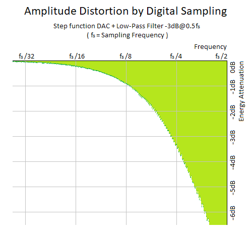
In this article, I simulated DAC generating step function signals followed by an analogue first-order low-pass filter with its cut-off at the Nyquist frequency. The plot shows the average energy of the regenerated output analogue signal compared to the original conceptual sine wave to be sampled.

As I argued before, and some of audiophiles believe, the 24/192 satisfies the 1dB distortion threshold. To satisfy 1% (0.08dB) distortion threshold, we need to go 24/768. Remember that the human hearing function is not that attenuated at the higher frequency.

We can display frequency response of the low-pass filter we applied layered over the plot as orange. However, be careful that you cannot divide the attenuation into the contribution from the filter and the theoretical contribution. If you do a little thought experiment, you can easily realise that the theory already says that the maximum attenuation at fs/4 is -3dB, which is close to the total attenuation in the plot. The additional attenuation comes from the shape smoothing from the step-shaped original wave shape.


Tuesday, 31 August 2021

Self-research: Why hi-res sounds better? Suggestion to prove hi-res hearing theory

Some audiophiles and companies like Sony argue that high resolution audio matters while others argue that those are indistinguishable. These arguments can only be proven by statistics on blind tests. Some tests suggests that some people seems indeed distinguishes high resolution sources. Audio experts says that this is because the mixing and mastering target between CD sources and hi-res sources are different; they made to sound differently in the first place. I do personally believe the utility of the high resolution audio not only for mixing purpose but also for listening purpose. (For processing audio, hi-res definitely helps to reduce distortion. Digital filters is distorted heavily near the Nyquist frequency.) But I am not arguing that we can hear beyond 24kHz. ( Indeed some people can hear 24kHz but no beyond.) I am arguing that we need infinitely high digital sampling rate to reproduce 20Hz-24kHz analog signal.

  Think about 24kHz signal in 48kHz sampling. If the phase is shifted pi/2, the signal is shown as 0. The digital sampling with frequency in the last octave under the Nyquist frequency only has peak samples, so there is almost zero reproducibility concerning phase shift. Even if the frequency of the signal is not a divisor of the sampling frequency, ghost beating sound is produced. So, in CD Sound, 10-20kHz sound is not well reproduced and has no meaning unless it is harmonics of another lower sounds.

  2nd last octave sound under the Nyquist has a sample middle of the curve, so at least we can guarantee that 1/sqrt(2) of the amplitude of the original sound can be reproduced. (Or, maybe we can expect better by physical low-pass filter.) So on for the higher…

What I really recommend is to play 24/192 or at least 24/96 with 20khz lp filter.

So, I suggest an experiment to compare not only between different sources on the same player, but also between different lp filter but using the same hi-res source and the same DAC. If my theory is right, Sony’s hi-res capability issue of speakers are useless, but hi-res for DAC is important.

I have no professional background on this, so I dont know whether people already know this. I think my story makes sense physically, so most specialists maybe already know this.

But the reason I am raising this as problem is that I dont understand why Sony counts speaker’s reproducibility of 40khz signal. I know that there is meaning to have flatter FR in audible frequencies generally when we demand hi-res capability of analog device. But is there more meaning over that?

 http://archimago.blogspot.com/2016/07/musings-digital-interpolation-filters.html

https://en.wikipedia.org/wiki/Bilinear_transform

Thursday, 8 April 2021

IEC Standard Weightings

Transfer functions:

\(H_A(s)=\dfrac{(12194\,\mathrm{Hz})^2\:\left(\frac{s}{2\pi}\right)^4\:\big/\: e^{-2.0000/20}}{(\frac{s}{2\pi}+20.6\,\mathrm{Hz})^2\,(\frac{s}{2\pi}+107.7\,\mathrm{Hz})\,(\frac{s}{2\pi}+ 737.9\,\mathrm{Hz})\,(\frac{s}{2\pi}+12194\,\mathrm{Hz})^2}\)

\(H_B(s)=\dfrac{(12194\,\mathrm{Hz})^2\:\left(\frac{s}{2\pi}\right)^3\:\big/\:  e^{-0.1697/20}}{\left(\frac{s}{2\pi}+20.6\,\mathrm{Hz}\right)^2\:\left(\frac{s}{2\pi}+158.5\,\mathrm{Hz}\right)\:\left(\frac{s}{2\pi}+12194\,\mathrm{Hz}\right)^2}\)

\(H_C(s)=\dfrac{(12194\,\mathrm{Hz})^2\:\left(\frac{s}{2\pi}\right)^2\:\big/\:  e^{-0.0619/20}}{\left(\frac{s}{2\pi}+20.6\,\mathrm{Hz}\right)^2\:\left(\frac{s}{2\pi}+12194\,\mathrm{Hz}\right)^2}\)

\(H_Z(s)=\dfrac{(2\pi\cdot 46066\,\mathrm{Hz})^2\:s^2}{(s+2\pi\cdot 4.34\,\mathrm{Hz})^2\:(s+2\pi\cdot 46066\,\mathrm{Hz})^2}\)

\(H_K(s)=\dfrac{1.5848634463348217\,s^2+18886.914378028894\,s+1.1260607147003824\times10^8}{s^2+15004.846526655707\,s+1.1259450726979023\times10^8}\)

\(\times\dfrac{1.0049948987146884\,s^2}{s^2+478.91221140843305\, s+57414.259359025615}\times 10^{-0.691/20}\)

\(\times\dfrac{(2\pi\cdot 46066\,\mathrm{Hz})^2}{(s+2\pi\cdot 46066\,\mathrm{Hz})^2}\)

*only A,C,K are standard

For RMS, after squaring, averaging technique may be RC LP filter.

for VU meter standard, RC = 0.0651442s equiv 2.44312 Hz

for loudness RMS (LKFS standard) RC = 0.392323 equiv 0.405674 Hz

https://en.wikipedia.org/wiki/A-weighting

https://www.itu.int/dms_pubrec/itu-r/rec/bs/R-REC-BS.1770-3-201208-S!!PDF-E.pdf

https://www.dsprelated.com/freebooks/filters/Low_High_Shelving_Filters.html

https://en.wikipedia.org/wiki/LKFS